Simulation Tutorial¶

[1]:

import PyPWA as pwa
import numpy as npy
import pandas
import matplotlib.pyplot as plt
import warnings
warnings.filterwarnings('ignore')

Define (import) amplitude (function) to simulate¶

The function will be use by the rejection method to “carve” a new distribution into the input simulated data read in next lines.

[2]:

#
import AmplitudeJPACsim
amp = AmplitudeJPACsim.NewAmplitude()

Read input (flat) simulated data (in condense format)¶

[3]:

data = pwa.read("etapiHEL2_flat.txt")

Read data full (from gamp files)

[4]:

datag = pwa.read("../TUTORIAL_FILES/raw_events.gamp")

The format of the input data will depend on the Amplitudes: In this example the standard HEL angles, polarization angle (alpha) and other information neccesary are given for PWA (see below)

[5]:

data

[5]:

	EventN	theta	phi	alpha	pol	tM	mass
0	0.0	1.902160	3.800470	-1.074900	0.4	-0.026354	0.850234
1	1.0	0.916137	1.660230	-1.438370	0.4	-0.671785	2.619530
2	2.0	1.811330	5.778960	-2.341440	0.4	-0.077582	1.268280
3	3.0	2.000940	5.250000	2.709120	0.4	-0.726730	1.253960
4	4.0	1.871130	2.697150	0.239302	0.4	-0.156830	0.927206
...	...	...	...	...	...	...	...
9855141	9855141.0	1.354170	5.931830	0.784408	0.4	-0.054668	1.083350
9855142	9855142.0	2.335000	3.347330	-0.748025	0.4	-0.844509	1.483240
9855143	9855143.0	1.328470	1.948730	-2.102880	0.4	-0.138508	0.940464
9855144	9855144.0	2.184290	2.491810	-1.821200	0.4	-0.314037	0.723398
9855145	9855145.0	1.570570	0.590933	-1.335300	0.4	-0.240994	1.187410

9855146 rows × 7 columns

Produce simulation mask¶

A boolean file of (False and True)

[6]:

rejection = pwa.monte_carlo_simulation(amp, data, dict(), 16)

Check on the waves and resonances that will be produced > This is a matrix with the weigths of each wave on each resonance

[7]:

amp.setup(data)
table =[]
tabler=[]

for r in range(amp.resonance.resonance_index):
    tabler.append(amp.resonance.W0[r])
    tabler.append(amp.resonance.Cr[r])
    for w in range(amp.resonance.wave_index):

        tabler.append(amp.resonance.Wave[r][w])
    table.append(tabler)
    tabler=[]

from tabulate import tabulate
headers=["Resonance","Res-weight"]
for w in range(amp.resonance.wave_index):
    headers.append(amp.resonance.wave_data[w])

print(tabulate(table,headers))

  Resonance    Res-weight    (1, 0, 0)    (1, 1, 0)    (1, 1, -1)    (1, 1, 1)    (1, 2, 0)    (1, 2, -1)    (1, 2, 1)    (1, 2, -2)    (1, 2, 2)
-----------  ------------  -----------  -----------  ------------  -----------  -----------  ------------  -----------  ------------  -----------
      0.98           0.65            1          0               0          0           0                0         0                0         0
      1.306          0.35            0          0               0          0           0.33             0         0.33             0         0.33
      1.584          0.08            0          0.5             0          0.5         0                0         0                0         0
      1.722          0.1             0          0               0          0           0.33             0         0.33             0         0.33

Check on how many events will be kept through the masking

[8]:

print(f"Removed {len(data) - npy.sum(rejection)} events from flat data.")
print(f"Kept {npy.sum(rejection)} events.")
print(f"{(npy.sum(rejection) / len(data)) * 100}% of events remain.")

Removed 9454013 events from flat data.
Kept 401133 events.
4.070289775514234% of events remain.

Apply mask to input data¶

new_data will contain the simulated data in the same format that data/datag

[9]:

new_data = data[rejection]

[10]:

new_data

[10]:

	EventN	theta	phi	alpha	pol	tM	mass
137	137.0	2.206940	1.953870	-0.247381	0.4	-0.120428	0.995635
171	171.0	1.775060	1.264290	2.600410	0.4	-0.345176	1.167540
200	200.0	0.128817	2.396510	-0.063606	0.4	-0.229984	2.269060
205	205.0	0.696665	1.981680	3.079090	0.4	-0.184068	1.885680
237	237.0	1.051710	1.753500	-2.496390	0.4	-1.500240	1.334010
...	...	...	...	...	...	...	...
9855028	9855028.0	0.858080	2.779910	-0.051326	0.4	-0.086823	0.981714
9855041	9855041.0	1.620860	0.822745	1.592530	0.4	-0.451578	1.311310
9855064	9855064.0	0.734074	5.887190	-1.768290	0.4	-0.099859	1.098970
9855075	9855075.0	1.502800	1.512360	0.860545	0.4	-0.162814	1.710660
9855113	9855113.0	1.324710	4.971240	-1.140430	0.4	-0.051079	1.154320

401133 rows × 7 columns

Mask full data format

[11]:

new_datag = datag[rejection]

Write new_data into a Pandas Dateframe

[12]:

amp.setup(new_data)
new_data = pandas.DataFrame(new_data)

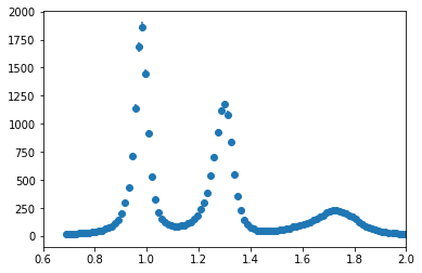
Plot simulated data intensity versus mass¶

[13]:

results = amp.calculate()
mni = npy.empty(len(new_data), dtype=[("mass", float), ("intensity", float)])
mni["mass"] = new_data["mass"]
mni["intensity"] = results.real
mni = pandas.DataFrame(mni)
counts, bin_edges = npy.histogram(mni["mass"], 200, weights=mni["intensity"])
centers = (bin_edges[:-1] + bin_edges[1:]) / 2

# Add yerr to argment list when we have errors
yerr = npy.empty(100)
yerr = npy.sqrt(counts)
plt.errorbar(centers,counts, yerr, fmt="o")
#plt.yscale("log")
plt.xlim(.6, 2.)

[13]:

(0.6, 2.0)

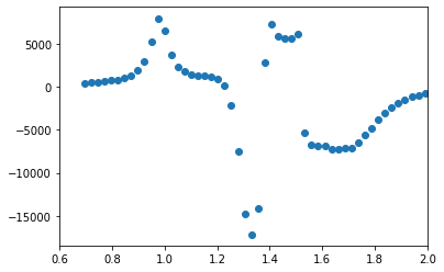
../_images/examples_demo_JPAC_sim_24_1.png

Calculate Phase difference between two waves¶

In this example first and 3erd waves in amplitude list

[14]:

#if amp.Vs[1]15].all() != 0 and amp.Vs[0][0].all() != 0:
phasediff = npy.arctan(npy.imag(amp.Vs[2][3]*amp.Vs[1][6].conjugate())/npy.real(amp.Vs[2][3]*amp.Vs[1][6].conjugate()))
#phasediff = npy.arctan(npy.imag(amp.Vs[2][1]*amp.Vs[1][2].conjugate())/npy.real(amp.Vs[2][1]*amp.Vs[1][2].conjugate()))

Plot PhaseMotion

[15]:

mnip = npy.empty(len(new_data), dtype=[("mass", float), ("phase", float)])
mnip["mass"] = new_data["mass"]
mnip["phase"] = phasediff
mnip = pandas.DataFrame(mnip)
counts, bin_edges = npy.histogram(mnip["mass"], 100, weights=mnip["phase"])
centers = (bin_edges[:-1] + bin_edges[1:]) / 2

# Add yerr to argment list when we have errors
yerr = npy.empty(100)
yerr = npy.sqrt(counts)
plt.errorbar(centers,counts, yerr, fmt="o")
plt.xlim(0.6, 2.)

[15]:

(0.6, 2.0)

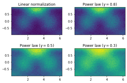
../_images/examples_demo_JPAC_sim_28_1.png

Plot phi_HEL vs cosHEL) of simulated data (with 4 different contracts(gamma))

[16]:

import matplotlib.colors as mcolors
from numpy.random import multivariate_normal

gammas = [0.8, 0.5, 0.3]

fig, axes = plt.subplots(nrows=2, ncols=2)

axes[0, 0].set_title('Linear normalization')
axes[0, 0].hist2d(new_data["phi"], npy.cos(new_data["theta"]), bins=100)
#axes[0, 0].hist2d(cut_list["phi"], npy.cos(cut_list["theta"]), bins=100)

for ax, gamma in zip(axes.flat[1:], gammas):
    ax.set_title(r'Power law $(\gamma=%1.1f)$' % gamma)
    ax.hist2d(new_data["phi"], npy.cos(new_data["theta"]),
        bins=100, norm=mcolors.PowerNorm(gamma))

fig.tight_layout()

plt.show()

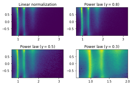
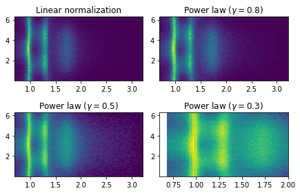
../_images/examples_demo_JPAC_sim_30_0.png

Plot cos(theta_HEL) vs mass for simulated data (with 4 different contrasts)

[17]:

gammas = [0.8, 0.5, 0.3]

fig, axes = plt.subplots(nrows=2, ncols=2)

axes[0, 0].set_title('Linear normalization')
axes[0, 0].hist2d(new_data["mass"], npy.cos(new_data["theta"]),bins=100)

for ax, gamma in zip(axes.flat[1:], gammas):
    ax.set_title(r'Power law $(\gamma=%1.1f)$' % gamma)
    ax.hist2d(new_data["mass"], npy.cos(new_data["theta"]),
              bins=100, norm=mcolors.PowerNorm(gamma))


fig.tight_layout()
plt.xlim(.6, 2.)
plt.show()

../_images/examples_demo_JPAC_sim_32_0.png

Plot phiHEL vs mass for simulated data (with 4 different contrasts)

[18]:

gammas = [0.8, 0.5, 0.3]

fig, axes = plt.subplots(nrows=2, ncols=2)

axes[0, 0].set_title('Linear normalization')
axes[0, 0].hist2d(new_data["mass"], new_data["phi"],bins=100)

for ax, gamma in zip(axes.flat[1:], gammas):
    ax.set_title(r'Power law $(\gamma=%1.1f)$' % gamma)
    ax.hist2d(new_data["mass"], new_data["phi"],
              bins=100, norm=mcolors.PowerNorm(gamma))


fig.tight_layout()
plt.xlim(.6, 2.)
plt.show()

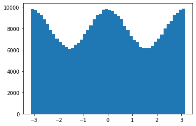
../_images/examples_demo_JPAC_sim_34_0.png

Histogram of alpha/Phi > alpha/Phi is the polarization angle

[19]:

plt.hist(new_data["alpha"],50)
plt.show()

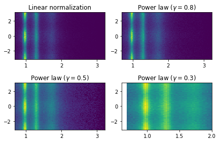
../_images/examples_demo_JPAC_sim_36_0.png

Plot mass versus alpha/Phi

[20]:

gammas = [0.8, 0.5, 0.3]

fig, axes = plt.subplots(nrows=2, ncols=2)

axes[0, 0].set_title('Linear normalization')
axes[0, 0].hist2d(new_data["mass"], new_data["alpha"],bins=100)

for ax, gamma in zip(axes.flat[1:], gammas):
    ax.set_title(r'Power law $(\gamma=%1.1f)$' % gamma)
    ax.hist2d(new_data["mass"], new_data["alpha"],
              bins=100, norm=mcolors.PowerNorm(gamma))


fig.tight_layout()
plt.xlim(.6, 2.)
plt.show()

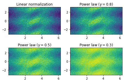
../_images/examples_demo_JPAC_sim_38_0.png

Plot phi_HEL versus alpha/Phi

[21]:

gammas = [0.8, 0.5, 0.3]

fig, axes = plt.subplots(nrows=2, ncols=2)

axes[0, 0].set_title('Linear normalization')
axes[0, 0].hist2d(new_data["phi"],new_data["alpha"],bins=100)

for ax, gamma in zip(axes.flat[1:], gammas):
    ax.set_title(r'Power law $(\gamma=%1.1f) $' % gamma)
    ax.hist2d(new_data["phi"], new_data["alpha"],
              bins=100, norm=mcolors.PowerNorm(gamma))


fig.tight_layout()

plt.show()

../_images/examples_demo_JPAC_sim_40_0.png

Write simulated data to disk¶

[23]:

new_data.to_csv("simdata_JPAC.csv", index=False)

Write gamp data after maked

[24]:

pwa.write("raw_simulated_JPAC.gamp",new_datag)

Calculate Moments (for JPAC or Std) and Asymmetries¶

[25]:

H000,H010,H011,H020,H021,H022,H100,H110,H111,H120,H121,H122,sigma4,sigmay = amp.calculate_moments_JPAC()
#H00,H11,H10,H20,H21,H22 = amp.calculate_moments_STD()

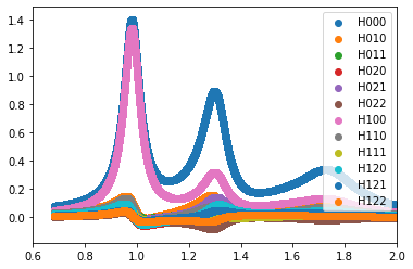
Plot (all) Moments versus mass

[26]:

plt.scatter(new_data["mass"],H000,LABEL="H000")
plt.legend(loc='upper right')
plt.scatter(new_data["mass"],H010,LABEL="H010")
plt.legend(loc='upper right')
plt.scatter(new_data["mass"],H011,LABEL="H011")
plt.legend(loc='upper right')
plt.scatter(new_data["mass"],H020,LABEL="H020")
plt.legend(loc='upper right')
plt.scatter(new_data["mass"],H021,LABEL="H021")
plt.legend(loc='upper right')
plt.scatter(new_data["mass"],H022,LABEL="H022")
plt.legend(loc='upper right')
plt.scatter(new_data["mass"],H100,LABEL="H100")
plt.legend(loc='upper right')
plt.scatter(new_data["mass"],H110,LABEL="H110")
plt.legend(loc='upper right')
plt.scatter(new_data["mass"],H111,LABEL="H111")
plt.legend(loc='upper right')
plt.scatter(new_data["mass"],H120,LABEL="H120")
plt.legend(loc='upper right')
plt.scatter(new_data["mass"],H121,LABEL="H121")
plt.legend(loc='upper right')
plt.scatter(new_data["mass"],H122,LABEL="H122")
plt.legend(loc='upper right')
plt.xlim(0.6, 2.)

[26]:

(0.6, 2.0)

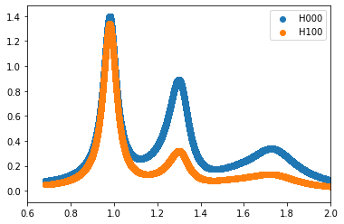
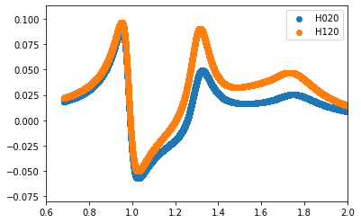
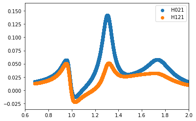
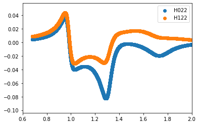
../_images/examples_demo_JPAC_sim_48_1.png

PLot each moment vs mass

[27]:

plt.xlim(0.6, 2.)
plt.scatter(new_data["mass"],H000,LABEL="H000")
plt.scatter(new_data["mass"],H100,LABEL="H100")
plt.legend(loc='upper right')
plt.show()
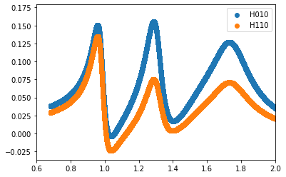
plt.xlim(0.6, 2.)
plt.scatter(new_data["mass"],H010,LABEL="H010")
plt.scatter(new_data["mass"],H110,LABEL="H110")
plt.legend(loc='upper right')
plt.show()
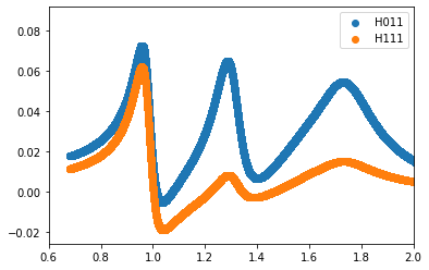
plt.xlim(0.6, 2.)
plt.scatter(new_data["mass"],H011,LABEL="H011")
plt.scatter(new_data["mass"],H111,LABEL="H111")
plt.legend(loc='upper right')
plt.show()
plt.xlim(0.6, 2.)
plt.scatter(new_data["mass"],H020,LABEL="H020")
plt.scatter(new_data["mass"],H120,LABEL="H120")
plt.legend(loc='upper right')
plt.show()
plt.xlim(0.6, 2.)
plt.scatter(new_data["mass"],H021,LABEL="H021")
plt.scatter(new_data["mass"],H121,LABEL="H121")
plt.legend(loc='upper right')
plt.show()
plt.xlim(0.6, 2.)
plt.scatter(new_data["mass"],H022,LABEL="H022")
plt.scatter(new_data["mass"],H122,LABEL="H122")
plt.legend(loc='upper right')
plt.show()

../_images/examples_demo_JPAC_sim_50_0.png

../_images/examples_demo_JPAC_sim_50_1.png

../_images/examples_demo_JPAC_sim_50_2.png

../_images/examples_demo_JPAC_sim_50_3.png

../_images/examples_demo_JPAC_sim_50_4.png

../_images/examples_demo_JPAC_sim_50_5.png

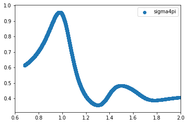
Plot asymmetry Sigma_4PI

[28]:

plt.xlim(0.6, 2.)
plt.scatter(new_data["mass"],sigma4,LABEL="sigma4pi")
plt.legend(loc='upper right')
plt.show()

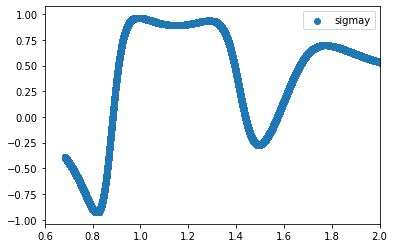
../_images/examples_demo_JPAC_sim_52_0.png

Plot asymmetry Sigma_y

[29]:

plt.xlim(0.6, 2.)
plt.scatter(new_data["mass"],sigmay,LABEL="sigmay")
plt.legend(loc='upper right')

[29]:

<matplotlib.legend.Legend at 0x7f0c54a93390>

../_images/examples_demo_JPAC_sim_54_1.png

[ ]: