Prediction Tutorial¶

Simulates “true data” corrected by acceptance, according to

the fitted values for the amplitude

[1]:

import PyPWA as pwa
import numpy as npy
import pandas
import matplotlib.pyplot as plt
import warnings
warnings.filterwarnings('ignore')

Define waves and amplitude (function) to simulate¶

[2]:

initial=[]
for param_type in ["r", "i"]:
    initial.append(f"{param_type}.1.0.0")
    initial.append(f"{param_type}.1.1.0")
    initial.append(f"{param_type}.1.1.1")
    initial.append(f"{param_type}.1.2.0")
    initial.append(f"{param_type}.1.2.1")
    initial.append(f"{param_type}.1.2.2")
#import AmplitudeOLDfit
#amp = AmplitudeOLDfit.FitAmplitude(initial)
#
import AmplitudeJPACsim
amp = AmplitudeJPACsim.NewAmplitude()
#
#import AmplitudeJPACfit
#amp = AmplitudeJPACfit.FitAmplitude(initial)

Read input (flat) simulated (generated) data¶

[3]:

data = pwa.read("etapiHEL_flat.txt")

Read flat data in gamp format (full information)

[4]:

datag = pwa.read("../TUTORIAL_FILES/raw_events.gamp")

Define number of bins (MUST be the same as the fitted parameters)

[5]:

nbins=20
bins = pwa.bin_by_range(data, "mass", nbins, .6, 2.0)

Calculate the mass value and number of events in each bin

[6]:

bmass=[]
mcounts=[]
for index, bin in enumerate(bins):
    if len(bin)==0:
        bmass.append(0.)
        mcounts.append(0.)
    else:
        bmass.append(npy.average(bin["mass"]))
        mcounts.append(len(bin))

Read parameters from fit¶

[7]:

par = pwa.read("final_values_JPAC.csv")

Prepare for a binned simulation > Find intensities in each bin and max intensity for each bin.

[8]:

int_values = []
max_values = []
params={}
for index, bin in enumerate(bins):
    for param_type in ["r", "i"]:
        params.update({f"{param_type}.1.0.0":par[f"{param_type}.1.0.0"][index]})
        params.update({f"{param_type}.1.1.0":par[f"{param_type}.1.1.0"][index]})
        params.update({f"{param_type}.1.1.1":par[f"{param_type}.1.1.1"][index]})
        params.update({f"{param_type}.1.2.0":par[f"{param_type}.1.2.0"][index]})
        params.update({f"{param_type}.1.2.1":par[f"{param_type}.1.2.1"][index]})
        params.update({f"{param_type}.1.2.2":par[f"{param_type}.1.2.2"][index]})


    [int,intmax] = pwa.simulate.process_user_function(amp,bin,params,16)
    int_values.append(int)
    max_values.append(intmax)

Simulate events for each bin (produce mask and mask them)¶

[9]:

rejected_bins = []
masked_final_values = []
for int_value, bin in zip(int_values, bins):
    rejection = pwa.simulate.make_rejection_list(int_value, max_values)
    rejected_bins.append(bin[rejection])
    masked_final_values.append(int_value[rejection])

Check how many events simulated by bin

[10]:

for index, simulated_bin in enumerate(rejected_bins):
    print(
        f"Bin {index+1}'s length is {len(simulated_bin)}, "
        f"{(len(simulated_bin) / len(bin)) * 100:.2f}% events were kept"
    )

Bin 1's length is 4850, 1.79% events were kept
Bin 2's length is 6545, 2.42% events were kept
Bin 3's length is 10388, 3.84% events were kept
Bin 4's length is 25492, 9.42% events were kept
Bin 5's length is 65913, 24.34% events were kept
Bin 6's length is 27495, 10.15% events were kept
Bin 7's length is 15419, 5.69% events were kept
Bin 8's length is 17872, 6.60% events were kept
Bin 9's length is 31916, 11.79% events were kept
Bin 10's length is 45793, 16.91% events were kept
Bin 11's length is 20121, 7.43% events were kept
Bin 12's length is 10427, 3.85% events were kept
Bin 13's length is 10301, 3.80% events were kept
Bin 14's length is 12541, 4.63% events were kept
Bin 15's length is 15215, 5.62% events were kept
Bin 16's length is 18517, 6.84% events were kept
Bin 17's length is 17288, 6.39% events were kept
Bin 18's length is 12478, 4.61% events were kept
Bin 19's length is 8226, 3.04% events were kept
Bin 20's length is 5718, 2.11% events were kept

Stak data for all bins in one file (new_data)

[11]:

for index, the_bin in zip(range(len(rejected_bins)), rejected_bins):
    if index ==0:
        new_data=pandas.DataFrame(the_bin)

    new_data =  new_data.append(the_bin,ignore_index=True)

#print(new_data)

[12]:

new_data

[12]:

	EventN	theta	phi	alpha	pol	tM	mass
0	432.0	1.075030	3.11080	-2.279760	0.4	-0.036087	0.730692
1	3277.0	1.106290	1.62386	2.912540	0.4	-0.021695	0.706537
2	5034.0	2.092900	1.77176	-1.243810	0.4	-0.065768	0.730773
3	5547.0	0.201674	-1.60246	-1.418660	0.4	-0.028844	0.701134
4	6527.0	1.325940	3.00931	-1.637510	0.4	-0.023814	0.722924
...	...	...	...	...	...	...	...
387360	9849089.0	1.940630	-1.85137	1.307640	0.4	-0.521166	1.968390
387361	9851359.0	1.055120	-2.61521	-2.743190	0.4	-0.403025	1.960020
387362	9853817.0	0.189324	-1.00286	-1.850720	0.4	-0.370487	1.944500
387363	9854636.0	1.043920	2.97397	-0.604751	0.4	-0.325758	1.971750
387364	9854972.0	0.607401	-1.62378	-1.638410	0.4	-0.282602	1.978580

387365 rows × 7 columns

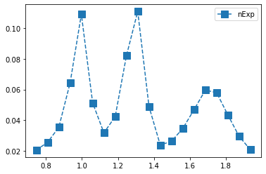
Calculate the number of expected events versus mass bins¶

[13]:

total_nExp = npy.empty(len(rejected_bins))
for index, the_bin in zip(range(len(rejected_bins)), rejected_bins):

    for param_type in ["r", "i"]:
        params.update({f"{param_type}.1.0.0":par[f"{param_type}.1.0.0"][index]})
        params.update({f"{param_type}.1.1.0":par[f"{param_type}.1.1.0"][index]})
        params.update({f"{param_type}.1.1.1":par[f"{param_type}.1.1.1"][index]})
        params.update({f"{param_type}.1.2.0":par[f"{param_type}.1.2.0"][index]})
        params.update({f"{param_type}.1.2.1":par[f"{param_type}.1.2.1"][index]})
        params.update({f"{param_type}.1.2.2":par[f"{param_type}.1.2.2"][index]})
    amp.setup(the_bin)
    total_nExp[index] = npy.average(amp.calculate(params))

Plot number of true (100% acc) events versus mass

[14]:

mni = npy.empty(len(total_nExp), dtype=[("mass", float), ("int", float)])
mni["mass"] = bmass
mni["int"] = total_nExp
mni = pandas.DataFrame(mni)
counts, bin_edges = npy.histogram(mni["mass"], nbins, weights=mni["int"])

centers = (bin_edges[:-1] + bin_edges[1:]) / 2

# Add yerr to argment list when we have errors
yerr = npy.empty(nbins)
yerr = npy.sqrt(counts)
yerr=0.
plt.errorbar(centers,counts, yerr, fmt="s",linestyle="dashed",markersize='10',label="nExp")

#plt.xlim(.6, 3.2)
#plt.ylim(0.,65000)
plt.legend(loc='upper right')
plt.show()

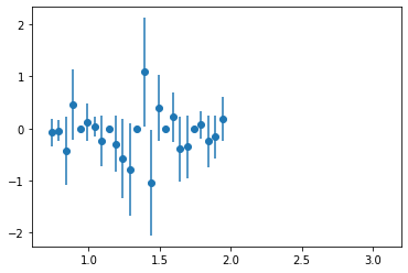
../_images/examples_demo_JPAC_pre_26_0.png

Calculate Phase difference between two waves¶

[15]:

V1=npy.ndarray(len(par))
V2=npy.ndarray(len(par))
V1 = par["r.1.1.1"]+par["i.1.1.1"]*(1j)
V2 = par["r.1.2.1"]+par["i.1.2.1"]*(1j)
if V1.all() != 0 and V2.all() != 0:
    phasediff = npy.arctan(npy.imag(V1*npy.conj(V2))/npy.real(V1*npy.conj(V2)))

Plot PhaseMotion

[16]:

mnip = npy.empty(len(bins), dtype=[("mass", float), ("phase", float)])
mnip["mass"] = bmass
mnip["phase"] = phasediff
mnip = pandas.DataFrame(mnip)
counts, bin_edges = npy.histogram(mnip["mass"], 25, weights=mnip["phase"])
centers = (bin_edges[:-1] + bin_edges[1:]) / 2

# Add yerr to argment list when we have errors
yerr = npy.empty(100)
yerr = npy.sqrt(npy.abs(counts))
plt.errorbar(centers,counts, yerr, fmt="o")
plt.xlim(0.6, 3.2)

[16]:

(0.6, 3.2)

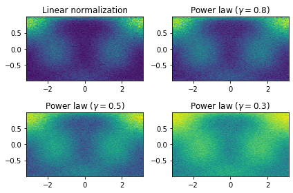
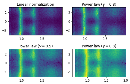
../_images/examples_demo_JPAC_pre_30_1.png

Plot phi_HEL vs cos(theta_HEL) of predicted data (with 4 different contracts(gamma))

[17]:

import matplotlib.colors as mcolors
from numpy.random import multivariate_normal

gammas = [0.8, 0.5, 0.3]

fig, axes = plt.subplots(nrows=2, ncols=2)

axes[0, 0].set_title('Linear normalization')
axes[0, 0].hist2d(new_data["phi"], npy.cos(new_data["theta"]), bins=100)
#axes[0, 0].hist2d(cut_list["phi"], npy.cos(cut_list["theta"]), bins=100)

for ax, gamma in zip(axes.flat[1:], gammas):
    ax.set_title(r'Power law $(\gamma=%1.1f)$' % gamma)
    ax.hist2d(new_data["phi"], npy.cos(new_data["theta"]),
        bins=100, norm=mcolors.PowerNorm(gamma))

fig.tight_layout()

plt.show()

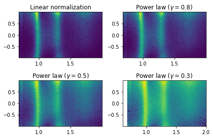
../_images/examples_demo_JPAC_pre_32_0.png

Plot cos(theta_HEL) vs mass for simulated data (with 4 different contrasts)

[18]:

gammas = [0.8, 0.5, 0.3]

fig, axes = plt.subplots(nrows=2, ncols=2)

axes[0, 0].set_title('Linear normalization')
axes[0, 0].hist2d(new_data["mass"], npy.cos(new_data["theta"]),bins=100)

for ax, gamma in zip(axes.flat[1:], gammas):
    ax.set_title(r'Power law $(\gamma=%1.1f)$' % gamma)
    ax.hist2d(new_data["mass"], npy.cos(new_data["theta"]),
              bins=100, norm=mcolors.PowerNorm(gamma))


fig.tight_layout()
plt.xlim(.6, 2.)
plt.show()

../_images/examples_demo_JPAC_pre_34_0.png

Plot phi_HEL vs mass for simulated data (with 4 different contrasts)

[19]:

gammas = [0.8, 0.5, 0.3]

fig, axes = plt.subplots(nrows=2, ncols=2)

axes[0, 0].set_title('Linear normalization')
axes[0, 0].hist2d(new_data["mass"], new_data["phi"],bins=100)

for ax, gamma in zip(axes.flat[1:], gammas):
    ax.set_title(r'Power law $(\gamma=%1.1f)$' % gamma)
    ax.hist2d(new_data["mass"], new_data["phi"],
              bins=100, norm=mcolors.PowerNorm(gamma))


fig.tight_layout()
plt.xlim(.6, 2.)
plt.show()

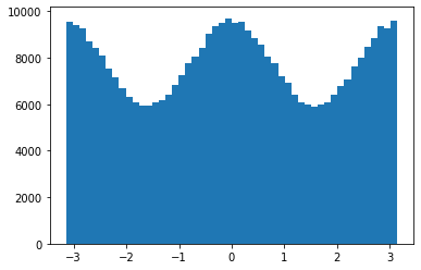
../_images/examples_demo_JPAC_pre_36_0.png

[ ]:

[20]:

plt.hist(new_data["alpha"],50)
plt.show()

../_images/examples_demo_JPAC_pre_38_0.png

Plot mass versus alpha/Phi

[21]:

gammas = [0.8, 0.5, 0.3]

fig, axes = plt.subplots(nrows=2, ncols=2)

axes[0, 0].set_title('Linear normalization')
axes[0, 0].hist2d(new_data["mass"], new_data["alpha"],bins=100)

for ax, gamma in zip(axes.flat[1:], gammas):
    ax.set_title(r'Power law $(\gamma=%1.1f)$' % gamma)
    ax.hist2d(new_data["mass"], new_data["alpha"],
              bins=100, norm=mcolors.PowerNorm(gamma))


fig.tight_layout()
plt.xlim(.6, 2.)
plt.show()

../_images/examples_demo_JPAC_pre_40_0.png

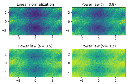
Plot mass versus alpha/Phi

[22]:

gammas = [0.8, 0.5, 0.3]

fig, axes = plt.subplots(nrows=2, ncols=2)

axes[0, 0].set_title('Linear normalization')
axes[0, 0].hist2d(new_data["phi"],new_data["alpha"],bins=100)

for ax, gamma in zip(axes.flat[1:], gammas):
    ax.set_title(r'Power law $(\gamma=%1.1f) $' % gamma)
    ax.hist2d(new_data["phi"], new_data["alpha"],
              bins=100, norm=mcolors.PowerNorm(gamma))


fig.tight_layout()

plt.show()

../_images/examples_demo_JPAC_pre_42_0.png

Write predicted (true) data to disk¶

[23]:

new_data.to_csv("predictedjpac.csv", index=False)

Write gamp format predicted to data (true)

[21]:

x = (data["EventN"]).astype(int)
y = (new_data["EventN"]).astype(int)

predm = npy.isin(x,y)
pdatag = datag[predm]
pwa.write("raw_predicted.gamp",pdatag)

Write predicted accepted data > events.pf is a mask of accepted data that has been produced by Geant

[24]:

acc = pwa.read("events.pf")
accn = acc.to_numpy()

mask_acc_phy = npy.logical_and(predm,accn)
pdatag_acc = datag[mask_acc_phy]
pdata_acc = data[mask_acc_phy]

pdata_acc.to_csv("predictedJPAC_ACC.csv", index=False)
pwa.write("acc_predictedJPAC.gamp",pdatag_acc)